How Deep Neural Networks Work

The advent of deep-learning-powered AI has changed the relation between humans and technology. Until now, we always had the possibility of referring to and relying on the knowledge and understanding of experts (or groups of experts) for information on even very advanced and complex pieces of technology. But in the case of deep learning technologies, not even machine learning experts have an end-to-end understanding of how exactly, i.e., according to which "learned" model these AIs process input and generate output. Is it ok for us to rely on the output of artificial intelligence, even when no one knows the underlying model the AI has employed to generate that output? This black box problem begs the question of whether it is ok for us to rely on the output of artificial intelligence, even when no one knows the underlying model the AI has employed to generate that output?

The black box problem affects all AI based on deep learning models, which are also the most powerful and prominent AIs out there, ranging from radiology CNNs to LLMs like ChatGPT. Since more and more people and companies are employing these AI tools, the black box problem will only affect more aspects of our life. This is what motivates our four-part "Can we trust black box AI?"-series.

Why talk about DNNs?

For illustrative purposes, we'll discuss the black box problem of AI by reference to the deep learning technology that has started the latest AI spring: Deep Neural Networks (or short: DNNs). In the late odds and early 2010s, DNNs started to surpass the performance of other, non-deep-learning forms of AI as well as the performance of manually programmed alternatives (Goodfellow, 2016). As of today, DNNs remain the core technology behind most of the latests innovations in AI.

DNN architecture

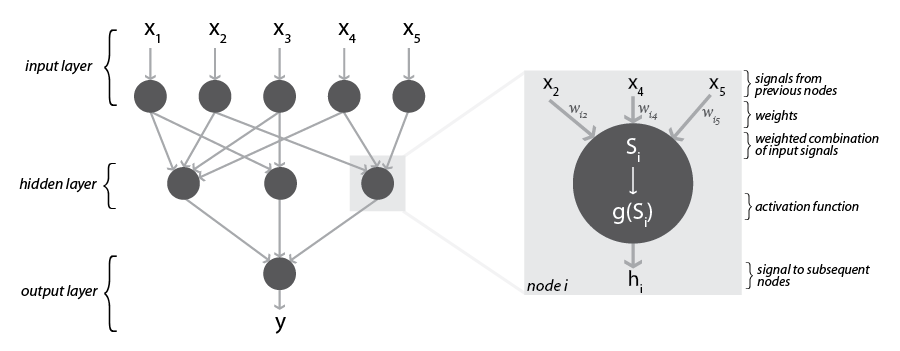Figure 1: Neural network with one hidden layer

The components of DNNs and linkages between them are “loosely inspired” (Goodfellow et al., 2016, p. 169) by neurons and synapses in the human and animal brain. As implementations in a DL software, DNNs consist of interconnected computational units, so-called nodes, which are arranged in at least three, but usually many more layers (up to 250, sometimes even more (Buckner, 2019, p. 3)): one input layer, followed by at least one, but usually multiple so-called hidden layers, and one output layer. A neuron in the input layer receives raw data as input (e.g., the pixel values of some section of an image) and transmits a numerical signal to those nodes in the next layer to which it is connected. The nodes in the first hidden layer take the signals from all the input nodes which they are connected to as inputs and transform them into an output signal, which they transmit to all the nodes in the following hidden layer to which they are connected. This process is repeated at every hidden layer until nodes of the last hidden layer transmit their numerical signals to the nodes in the output layer. The output nodes take these numerical signals as inputs and produce the final output. For an image classification task, the output might be a classification of an image as portraying a dog of a certain breed. Figure 1 depicts the general structure of a very simple three-layered neural net and the processing taking place at a node in the hidden layer. As illustrated here, DNNs used for image classification are usually sparsely, rather than fully, connected: the nodes of a hidden layer are only connected to some of the nodes in the previous and subsequent layer. This type of architecture makes the DNN’s training and application more efficient. Plus, models learned by sparsely-connected DNNs tend to generalize better to data outside the training set compared to models learned by fully-connected networks (Buckner, 2019, pp. 7–8).

What happens at the node level?

In order to transform the signals received from nodes of the previous layer into its own output, weights are assigned to the links between each pair of nodes. These weights determine by how much a node's signal will factor in the computation of the nodes in the subsequent layer. The exact way in which a node processes the weighted combination of the incoming signals is defined by its so-called activation function.

Typically, several activation functions are used throughout a DNN. In a DNN trained for image classification, for example, some nodes serve as filters, amplifying certain features while suppressing other features (convolutional nodes). Others detect whether a feature is present in a certain part of the data (rectified linear units). Nodes of yet another type aggregate information from previous nodes (maxpooling nodes) (Buckner, 2019).

Together, the incoming signals, the link weights and the activation function determine the activation level of a node. The node then transmits this activation level as output signal to those nodes in the subsequent layer to which it is connected. These nodes take the output of all their preceding nodes as input and repeat the process with their own weights. In this manner, the inputs are fed forward through the neural net until they reach the output layer, where the output nodes transform the signals they receive from the last hidden layer into the DNN’s final output. Consequently, different inputs, e.g., different images, will result in different activation levels at least for some of the nodes. If the activation pattern is different in a way that is relevant to the DNN’s decision model, the different inputs will result in different predictions or classifications.

Which DNN features are pre-determined by humans?

In setting up a DNN, the machine learning engineer determines–amongst other specifications–the number of layers, the number of nodes per layer, and with what kind of activation function nodes of a certain layer process their signals. What the ML engineer does not define, are the weights the nodes ultimately assign to incoming signals. The ML engineer merely assigns initial weights, which the DNN will adapt and overwrite itself during the training stage: training a DNN is essentially feeding the machine, or rather the model, data for which it learns the optimal weights.

Which DNN features are "learned"?

When DNNs employ Supervised Learning, their training set is labeled, i.e., it includes information on the actual class or outcome value associated with the input. During the learning process such a DNN compares its predicted output to this label and adjusts the weights connecting its nodes in a way that minimizes the so-called loss function. The loss function measures the divergence of predicted and actual outcome, e.g., the mean of squared errors. In order to adjust its model, the DNN first computes how it should change the weights on links connecting the output layer with the last hidden layer. Based on these results it then calculates the optimal adjustment for the weights connecting the last hidden layer with the second-to-last hidden layer, all the way to the weights of the links connecting the first hidden layer with the input layer.

The learning rate of a DNN, which determines how much the net adjusts its weights at each iteration, can be defined by the ML engineer before the training. Alternatively, the engineer can make it subject to dynamic optimization. In this case it varies depending on the improvement achieved through the preceding iteration. In each training iteration, the backpropagation algorithm calculates the gradient of the loss function w.r.t. the weights, whereas the adjustment algorithm, called gradient descent, is applied to adjust the weights such that the loss, the divergence of desired and predicted output, is minimized. It is through backpropagation/gradient descent that DNNs ‘learn’.

After the training stage, all weights, and thus, the DNN’s decision or prediction model remain fixed. Successfully training a DNN requires large amounts of data and computing power, which both have only become available during the last two decades. For instance, during training, the DNN-powered AlphaGo Zero has played 44 million games of Go against itself (Loo, 2021).

Why do DNNs perform so well?

Thanks to their deep structure, DNNs find representations of the data that facilitate pattern detection. Subsequent layers of a DNN use the representations of preceding layers to generate increasingly abstract and complex representations.

This hierarchical approach allows DNNs to approximate complex functions without requiring any pre-processed data (Buckner, 2019). In a DNN trained for image classification, early layers typically detect edges of particular angles in particular parts of the image, subsequent layers mute some of these particularities leading to increasing abstractions. Later layers combine edges, horizontal and vertical lines into small parts of objects, these to larger parts of objects and finally to entire objects which the machine then can classify. This architecture makes DNNs very sensitive to relevant variance in the data: DNNs can tell a white wolf from a Samoyed, a white dog bearing resemblance to wolves, even when they are both photographed in front of the same background and adopting the same posture (LeCun et al., 2015).

At the same time, DNNs are largely insensitive to noise, i.e., irrelevant variance in the input data. They can reliably recognize a Samoyed dog–regardless of lighting conditions, regardless of where in the picture the dog is located, regardless of whether the dog is sitting, lying, standing, or running. This combination of sensitivity to what matters and insensitivity to what does not produces a high level of accuracy in the predictions and classifications of DNNs (LeCun et al., 2015).

By 2015, DNNs trained on the ImageNet dataset (Russakovsky et al., 2015) classified images belonging to more than 1,000 categories slightly more accurately than Andrej Kaparthy, the only human who so far has committed to training his image recognition abilities with the ImageNet dataset. Kaparthy’s error rate in classifying images amounted to 5.1%. The error rate of humans who do not train with the ImageNet data before solving the classification task can go up to 15% (Kaparthy, 2014). Two years later, the error rate of DNNs dropped even more to below 3% (Langlotz et al., 2019). Particularly, when it comes to classifying images of a certain category into narrower sub-categories, DNNs, by now, can outperform humans: in a trial comparing human and DNN classification performance, the DNN correctly classified 99.46% percent of pictures of traffic signs in different environments and weather conditions. The best human participant correctly classified 99.22% of the pictures, the average correct classification rate of all humans came to 98.84% (Stallkamp et al., 2012).

References

Buckner, C. (2019): “Deep Learning: A Philosophical Introduction,” Philosophy Compass, 14, 1–19.
Goodfellow, I., Y. Bengio, A. Courville, and Y. Bengio (2016): Deep Learning, MIT Pess Cambridge.
Kaparthy, A. (2014-09-02): “What I Learned from Competing against a ConvNet on ImageNet,” Andrej Karpathy Blog.
Langlotz, C. P., B. Allen, B. J. Erickson, J. Kalpathy-Cramer, K. Bigelow, T. S. Cook, A. E. Flanders, M. P. Lungren, D. S. Mendelson, J. D. Rudie, et al. (2019): “A Roadmap for Foundational Research on Artificial Intelligence in Medical Imaging: from the 2018 NIH/RSNA/ACR/The Academy Workshop,” Radiology, 291, 781–791.
LeCun, Y., Y. Bengio, and G. Hinton (2015): “Deep Learning,” Nature, 521, 436– 444.
Loo, J. (2021-08-07): “The AI That Defeated Humans. Why We Don’t Stand a Chance,” Medium.
Russakovsky, O., J. Deng, H. Su, J. Krause, S. Satheesh, S. Ma, Z. Huang, A. Karpathy, A. Khosla, M. Bernstein, et al. (2015): “Imagenet Large Scale Visual Recognition Challenge,” International Journal of Computer Vision, 115, 211– 252.
Stallkamp, J., M. Schlipsing, J. Salmen, and C. Igel (2012): “Man vs. Computer: Benchmarking Machine Learning Algorithms for Traffic Sign Recognition,” Neural Networks, 32, 323–332.